A network estimate without stability checks is a hypothesis, not a finding. Two procedures — the nonparametric edge-weight bootstrap and the case-dropping subset bootstrap (summarized by the CS-coefficient) — tell you which parts of your network are signal and which are sampling noise. If a paper or a dashboard shows you a symptom network and neither of these appears anywhere, treat every “the strongest edge is…” and “the most central symptom is…” claim as provisional.

This is the fourth post in our methods series. We have covered why comorbidity motivates the network view, what centrality actually measures, and why EBICglasso estimates partial correlations. Today: the part that determines whether any of it is worth interpreting.

Why stability is the whole game

A regularized partial-correlation network is estimated from a sample. Every edge weight, and every centrality index derived from those weights, carries sampling variability — but the picture you get from qgraph looks deceptively exact. A node is drawn somewhere; an edge is drawn at some thickness. Nothing in the plot tells you that the third-strongest edge and the tenth-strongest edge might trade places in the next sample.

This is not a hypothetical worry. The replicability debate in network psychometrics (Forbes et al., 2017; and the replies that followed) turned largely on exactly this point: differences between networks that looked substantively meaningful were often within the range that sampling variability alone would produce. The constructive answer to that debate was not to abandon network estimation but to quantify the uncertainty routinely — which is what Epskamp, Borsboom, and Fried (2018) operationalized in the bootnet package.

Two different questions require two different bootstraps.

Question 1: How accurate are the edge weights?

The nonparametric bootstrap resamples your cases with replacement (typically 1,000+ times), re-estimates the network each time, and gives you a 95% confidence interval around every edge weight.

Reading these CIs correctly matters more than computing them:

• Wide CIs are the norm, not a failure. With realistic sample sizes, most edge CIs in a psychopathology network are wide. The question is whether they are wide relative to the differences you want to interpret.
• Overlapping CIs forbid ordering claims. If the CI of edge A overlaps substantially with the CI of edge B, you cannot claim A is “stronger” than B — even if the point estimates differ visibly in the plot. The bootstrapped difference test in bootnet makes this comparison explicit.
• CIs that cover a wide range around small estimates flag edges whose presence itself is uncertain. Regularization already shrinks weak edges toward zero, but survival of the LASSO is not proof of existence.

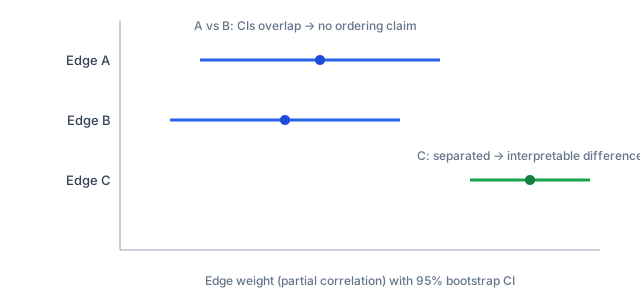
Point estimates suggest A > B, but their bootstrap CIs overlap heavily — the ordering is not supported. Only C is distinguishable from both.

Question 2: How stable are the centrality indices?

Edge CIs do not answer whether your centrality ranking would survive in a smaller sample. That is the job of the case-dropping subset bootstrap: re-estimate the network on progressively smaller subsets of your cases (90%, 70%, 50%…), compute centrality each time, and correlate those values with the full-sample centrality.

The CS-coefficient (correlation stability coefficient) summarizes the result: it is the largest proportion of cases you can drop while the correlation between subset and full-sample centrality stays ≥ 0.7 (with 95% certainty). Epskamp et al. (2018) proposed the working thresholds that the field has since adopted:

• CS ≥ 0.50 — the index is stable enough to interpret ordering.
• CS between 0.25 and 0.50 — interpret with caution; ordering claims are fragile.
• CS < 0.25 — do not interpret the ranking. Report it, and stop there.

Two patterns recur across published networks and are worth internalizing:

1. Strength and expected influence are usually the survivors. They aggregate over many edges, so noise in individual edges partially cancels.
2. Betweenness and closeness are usually the casualties. Both depend on shortest paths, and shortest paths are exquisitely sensitive to small perturbations in edge weights. A CS below 0.25 for betweenness is closer to the rule than the exception. If an interpretation hinges on a betweenness ranking with no reported CS, it hinges on very little.

The same logic extends to bridge centrality: bridge strength and bridge expected influence can be included in the case-dropping bootstrap (via the communities argument), and path-based bridge variants inherit the same fragility as their non-bridge counterparts.

A minimal, honest workflow

The entire accuracy pipeline is four calls in bootnet:

library(bootnet)

net <- estimateNetwork(data, default = "EBICglasso", tuning = 0.5)

# Q1 — edge-weight accuracy
boot_np <- bootnet(net, nBoots = 1000, type = "nonparametric")
plot(boot_np, labels = FALSE, order = "sample")   # edge CIs
plot(boot_np, "edge", plot = "difference")         # pairwise difference test

# Q2 — centrality stability
boot_case <- bootnet(net, nBoots = 2000, type = "case",
                     statistics = c("strength", "closeness",
                                    "betweenness", "expectedInfluence"))
corStability(boot_case)                            # CS-coefficients

Report all of it. A network paper — or any tool that visualizes networks for you — should surface (a) edge CIs, (b) the difference tests behind any ordering claim, and (c) CS-coefficients for every centrality index it displays. Where CS falls below 0.5, the honest move is to label the index as unstable in the same breath as showing it, not to bury the caveat in a supplement.

A reader’s checklist

When you encounter a symptom network in the wild, ask:

1. Was a bootstrap performed at all? Which types, how many iterations?
2. Are edge-ordering claims backed by the difference test, or just by point estimates?
3. Is a CS-coefficient reported for each centrality index that gets interpreted?
4. Are betweenness/closeness interpretations made despite CS < 0.25? (Red flag.)
5. Is the sample size plausible for the number of nodes? (A 9-node network needs to estimate 36 partial correlations; a 30-node network, 435.)

None of this makes network estimation fragile in some special, disqualifying way — every statistical model has sampling error. What bootnet did was make the uncertainty visible by default, and the field is better for it. A network with wide CIs and a low CS is not a failed analysis; it is an accurate report of how much this sample can tell you. The failed analysis is the one that never asked.

References

• Epskamp, S., Borsboom, D., & Fried, E. I. (2018). Estimating psychological networks and their accuracy: A tutorial paper. Behavior Research Methods, 50(1), 195–212.
• Epskamp, S., & Fried, E. I. (2018). A tutorial on regularized partial correlation networks. Psychological Methods, 23(4), 617–634.
• Forbes, M. K., Wright, A. G. C., Markon, K. E., & Krueger, R. F. (2017). Evidence that psychopathology symptom networks have limited replicability. Journal of Abnormal Psychology, 126(7), 969–988.
• Borsboom, D., Fried, E. I., Epskamp, S., Waldorp, L. J., van Borkulo, C. D., van der Maas, H. L. J., & Cramer, A. O. J. (2017). False alarm? A comprehensive reanalysis of “Evidence that psychopathology symptom networks have limited replicability.” Journal of Abnormal Psychology, 126(7), 989–999.