Series 11/13 · Book preview → Series hub
You have seen the picture. A ring of labelled circles, lines of varying thickness between them, two or three coloured clusters. It is the house style of network psychometrics, and for a sparse network of a dozen symptoms a flat qgraph layout is close to ideal. You take it in at a glance.
So why reach for a third dimension?
The honest answer is the unexciting one. A third dimension does not reveal anything the estimates did not already contain. The edges are the same regularised partial correlations (Epskamp, Borsboom & Fried, 2018); the centrality values are the same numbers. The structure lives in the estimates, not in the drawing — in 2D or 3D, the layout is only a way of displaying it.
What a third dimension changes is the room you have to display it in.
The flat diagram has a ceiling
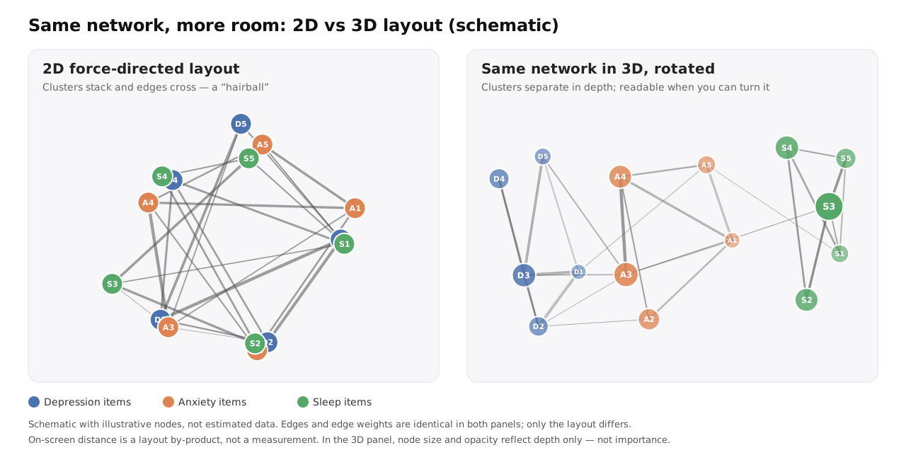
Most network figures use a force-directed layout, typically Fruchterman–Reingold (1991): connected nodes pull together, all nodes push apart, and the algorithm settles on a compromise in the plane. For a sparse graph, the plane is plenty. But add items, add scales, add the denser edge set you get when depression, anxiety and sleep items share one network, and the plane runs out of room. Nodes stack on nodes, edges cross edges, and three legible clusters collapse into what researchers call a “hairball.”
The network did not get worse; the drawing did. The information is intact, squeezed into a space too small to show it without overlap.
A third axis is one more degree of freedom for the same layout problem. Clusters that had to overlap on a plane can sit at different depths; edges that had to cross can pass over and under. It is not the only remedy — thresholding, faceting by scale, or multidimensional-scaling layouts that make 2D distance more meaningful (Jones, Mair & McNally, 2018) all help. It is one more option for when the graph is genuinely dense.
What 3D costs
Visualization researchers are rightly wary of 3D. Munzner (2014) states the rule bluntly: no unjustified 3D. Perspective shrinks distant objects, so size and length comparisons become unreliable; from any single viewpoint something is hidden behind something else; and a static screenshot of a 3D graph is often worse than a good 2D figure.
The justification, when there is one, comes from motion. Rotate a 3D graph and depth becomes readable through the kinetic depth effect — the way the eye separates foreground from background as things move. Experiments by Ware and colleagues found that motion and stereo depth cues helped people trace paths through graphs considerably larger than they could handle in 2D (Ware & Mitchell, 2008). The lesson is specific: 3D works when you can turn it. A 3D network you cannot rotate is mostly cost.
What 3D does not buy you
These limits matter more than the upside.
Screen distance is still not a measurement. In a spring layout, how far apart two nodes sit is a by-product of the algorithm, not a quantity you can read off (Jones, Mair & McNally, 2018). The same holds in 3D. If two nodes look close, that is a reason to check the edge between them, not a number in itself.
Centrality is read from the output, not the picture. A node is not more central because it landed in the visual middle or looks larger on screen. Centrality comes from the estimates, and should be read alongside edge-weight confidence intervals and a stability check such as the CS-coefficient (Epskamp, Borsboom & Fried, 2018) — with the known caveat that closeness and betweenness are often unstable in psychological networks (Bringmann et al., 2019).
None of it tells you what to do. A vivid, rotatable network is still a description of covariation in a reference sample. A central node is not, on that evidence alone, a treatment target; what centrality indices actually capture in these networks is itself under debate (Bringmann et al., 2019). And a structure estimated across many people describes that group, not the mechanism inside any one person — the two can genuinely diverge (Molenaar, 2004). A better picture does not relax these boundaries. A more persuasive picture asks for more discipline, not less.
Where 3D earns its place
Two places, honestly stated.
The first is exploring dense networks. When you can grab the graph and rotate it, clusters separate through motion, and a relationship buried under crossings on the page becomes something you can orbit and inspect. For a single sparse scale this is overkill. For a dense, multi-domain structure it can be the difference between a hairball and a readable object.
The second is engagement, used honestly. A network you can turn in your hands is easier to sit with than a static figure. That is not a scientific argument and I won’t dress it up as one — but for someone meeting symptom networks for the first time, “I can move it” lowers the cost of looking closely. The caveats travel with the image; the image just makes people more willing to read them.
Where this shows up in practice
This is the interaction model behind PsyNexa, the platform I am building. Reference networks render in the browser with Three.js: you rotate, zoom and bring a cluster toward you, and node labels are drawn to face the viewer so they stay readable from any angle. What the view offers is basic information for exploring a structure — not a verdict about it. The interpretation, and the responsibility for it, stay with the person reading.
Two dimensions did not fail us. They have a ceiling, and dense symptom networks are tall enough to hit it. The third dimension does not raise the truth. It raises the ceiling — at a price you pay back in motion.
References
- Bringmann, L. F., Elmer, T., Epskamp, S., Krause, R. W., Schoch, D., Wichers, M., Wigman, J. T. W., & Snippe, E. (2019). What do centrality measures measure in psychological networks? Journal of Abnormal Psychology, 128(8), 892–903.
- Epskamp, S., Borsboom, D., & Fried, E. I. (2018). Estimating psychological networks and their accuracy: A tutorial paper. Behavior Research Methods, 50(1), 195–212.
- Fruchterman, T. M. J., & Reingold, E. M. (1991). Graph drawing by force-directed placement. Software: Practice and Experience, 21(11), 1129–1164.
- Jones, P. J., Mair, P., & McNally, R. J. (2018). Visualizing psychological networks: A tutorial in R. Frontiers in Psychology, 9, 1742.
- Molenaar, P. C. M. (2004). A manifesto on psychology as idiographic science: Bringing the person back into scientific psychology, this time forever. Measurement: Interdisciplinary Research and Perspectives, 2(4), 201–218.
- Munzner, T. (2014). Visualization Analysis and Design. CRC Press.
- Ware, C., & Mitchell, P. (2008). Visualizing graphs in three dimensions. ACM Transactions on Applied Perception, 5(1), Article 2.