The short version: EBICglasso does not draw a network of correlations. It draws a network of regularized partial correlations — each edge is the association between two symptoms after conditioning on every other symptom in the model, shrunk toward zero by a lasso penalty whose strength is chosen by the Extended Bayesian Information Criterion. That one design choice — partial, not zero-order — is what makes the resulting graph interpretable as a map of direct relationships rather than a hairball of shared variance. The price: small true edges get erased, and edge weights are biased toward zero. Both the benefit and the cost are worth understanding before you trust any network figure, including ours.

In the previous post we ended with a promise: to open the box and look at what EBICglasso actually does — why partial correlations, why regularization, and what gets sacrificed. This is that post. Three minutes, one figure, no hand-waving.

The problem with raw correlations

Take nine depression symptoms (PHQ-9). Compute all pairwise correlations and draw an edge for each one. You will get a nearly complete graph: 36 possible edges, almost all of them positive and nonzero. Why? Because depressive symptoms share variance for many overlapping reasons — common causes, indirect chains, item overlap. A zero-order correlation between fatigue and concentration problems mixes together at least three things:

1. A possible direct relationship (being exhausted genuinely impairs concentration),
2. Indirect paths (fatigue → depressed mood → concentration), and
3. Shared causes elsewhere in the system (sleep disturbance driving both).

A network drawn from raw correlations cannot distinguish these. Every indirect path shows up as an edge, so the graph tells you little beyond “these symptoms co-occur” — which we already knew.

What a partial correlation is

The partial correlation between symptoms A and B is their association after statistically controlling for all other symptoms in the network. If the fatigue–concentration link survives conditioning on the other seven PHQ-9 items, that is evidence (not proof) of a direct dependency between them — a relationship not fully explained by the rest of the measured system.

Formally, under multivariate normality, partial correlations correspond (with a sign flip: −ω_ij/√(ω_iiω_jj)) to the off-diagonal elements of the standardized inverse covariance matrix (the precision matrix). A zero in the precision matrix means conditional independence: once you know the other variables, A tells you nothing further about B. This is the Gaussian graphical model (GGM), and it is the statistical object that psychometric “symptom networks” in the Borsboom–Cramer tradition actually estimate (Epskamp, Borsboom & Fried, 2018).

So the interpretive upgrade is real: edges in a GGM are candidates for direct relationships — pathways along which one symptom could plausibly influence another. That is precisely the reading the network theory of mental disorders needs.

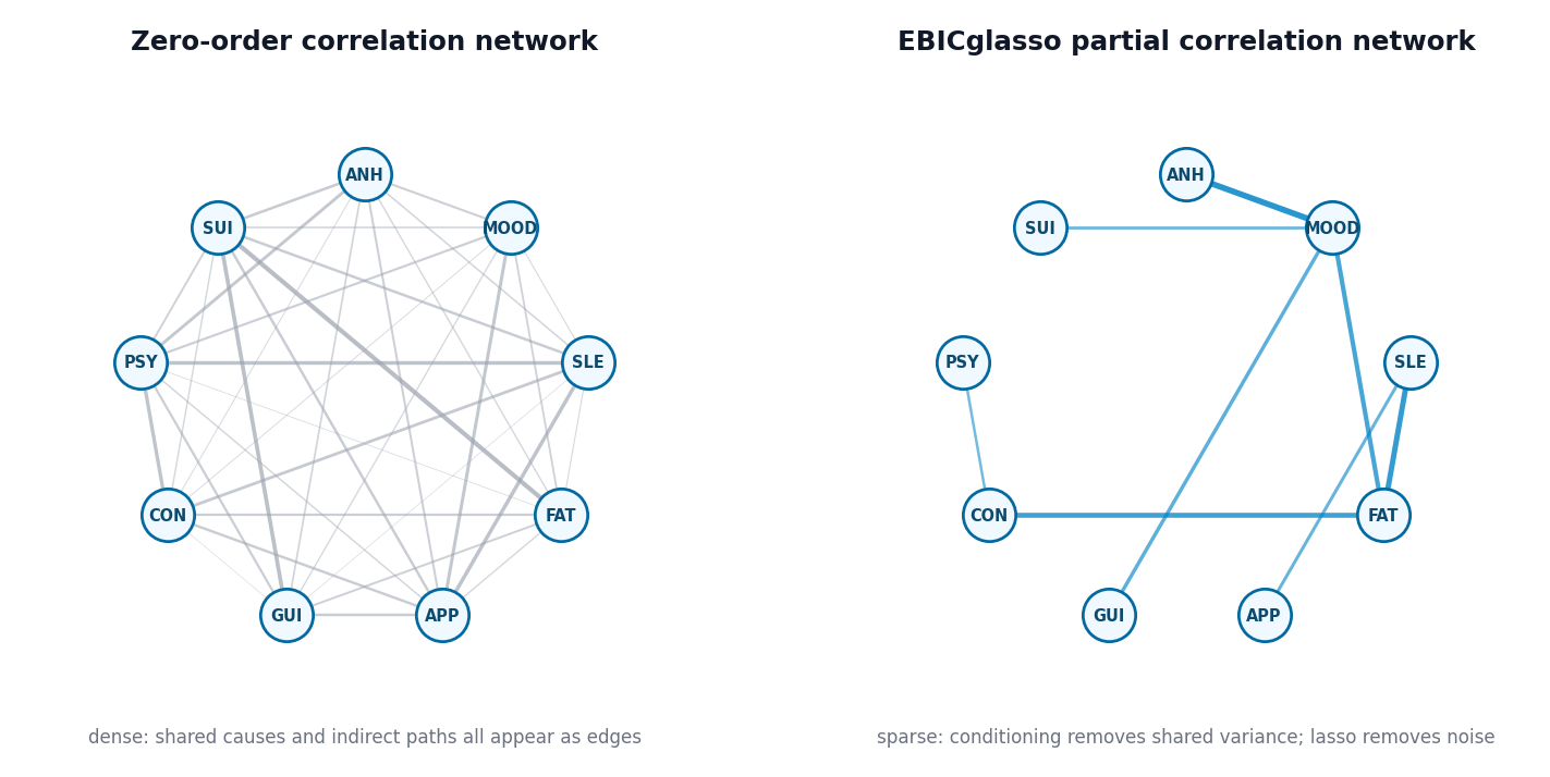
Figure 1. Same data, two graphs (synthetic illustration). Conditioning removes shared variance; regularization removes noise.

Why regularize at all?

Here is the catch. Sample partial correlations are noisy — with p variables you estimate p(p−1)/2 parameters, and with modest samples many of those estimates will be small but nonzero purely by chance. An unregularized partial correlation network is therefore also dense, just dense with noise instead of shared variance.

The graphical lasso (glasso; Friedman, Hastie & Tibshirani, 2008) fixes this by estimating the precision matrix under an L1 penalty: it maximizes the likelihood minus λ times the sum of absolute values of the entries. The L1 geometry has a distinctive consequence — it does not just shrink small estimates, it sets them to exactly zero. The result is a sparse network in which surviving edges have earned their place against a penalty.

Where EBIC comes in

The penalty λ is a dial: crank it up and the network gets emptier; turn it down and edges flood back. EBICglasso chooses λ by fitting a whole path of networks and selecting the one that minimizes the Extended BIC (Foygel & Drton, 2010, as implemented in qgraph). EBIC adds a hyperparameter γ (default 0.5 in qgraph/bootnet) that penalizes model complexity beyond ordinary BIC: higher γ prefers sparser, more conservative networks.

The design intent is asymmetric: EBICglasso with γ = 0.5 is tuned to favor specificity over sensitivity — it would rather miss a weak true edge than report a false one (Epskamp & Fried, 2018). For a field where network figures are read substantively, that is a defensible default: an edge you show should be an edge you can stand behind.

What you sacrifice

Nothing is free, and three costs matter in practice:

1. Small true edges disappear. The same conservatism that suppresses noise also erases genuinely weak dependencies. Absence of an edge in an EBICglasso network is not evidence of conditional independence — it may simply be an edge too weak to survive the penalty at your sample size.

2. Edge weights are biased toward zero. Lasso shrinkage means the plotted edge weights systematically understate the population partial correlations. Comparing raw edge weights across networks estimated on different samples is therefore riskier than it looks.

3. The result depends on estimation choices. γ, the correlation input (Pearson vs. polychoric via cor_auto), sample size, and even the number of nodes all shape which edges appear. Two labs analyzing similar data with different defaults can publish visibly different networks. This is not a scandal; it is a reason to report your settings and to quantify stability — which is exactly where the next post is headed.

The R incantation, for the record

The entire pipeline above is three calls in R:

library(qgraph)
cors <- cor_auto(data)                     # polychoric-aware correlations
net  <- EBICglasso(cors, n = nrow(data),   # glasso path + EBIC selection
                   gamma = 0.5)
qgraph(net, layout = "spring")             # the familiar figure

Every network figure we publish is generated by this family of tools (qgraph, bootnet), from public data, with sources and settings stated — because in this literature, the estimation choices are part of the result.

What’s next

A sparse, regularized network answers “which edges survive?” but not “how much should I trust them?” The next post covers the second question: bootstrapped confidence intervals and the CS-coefficient — the difference between a network that is a finding and a network that is a Rorschach test.

---

This post describes network structures; it is not diagnostic guidance or treatment recommendation.

References

• Epskamp, S., Borsboom, D., & Fried, E. I. (2018). Estimating psychological networks and their accuracy: A tutorial paper. Behavior Research Methods, 50(1), 195–212.
• Epskamp, S., & Fried, E. I. (2018). A tutorial on regularized partial correlation networks. Psychological Methods, 23(4), 617–634.
• Friedman, J., Hastie, T., & Tibshirani, R. (2008). Sparse inverse covariance estimation with the graphical lasso. Biostatistics, 9(3), 432–441.
• Foygel, R., & Drton, M. (2010). Extended Bayesian information criteria for Gaussian graphical models. Advances in Neural Information Processing Systems, 23.